
3D Annotation#
FiftyOne Enterprise lets you view and annotate 3D scenes recorded by a vehicle or robot: LiDAR point clouds, calibrated camera images, and the 3D labels that tie them together. You draw cuboids and polylines in the 3D tile, follow objects through time as tracks on the timeline, and see every edit projected onto the camera images as you work.
In the video, four 3D tiles show one frame: an Orbit view, a Cuboid top view and two camera views. A cuboid drawn in the front-right camera moves and resizes in all four at once. Every 3D tile is a full editor, camera views included.
Note
The screenshots and videos on this page use PandaSet by Scale AI and Hesai, licensed under CC BY 4.0.
This page follows the two people who work with 3D scenes:
Dataset owners load recordings with the Python SDK and make them playable. Start at How to: Prepare a 3D dataset.
Annotators view scenes and label them in the App. Start at How to: View a 3D scene.
How 3D scenes work#
Scene (dynamic group) ─── Frame (group) ─┬─ LiDAR slice ─── point cloud, cuboids, polylines
                                         └─ camera slices ── images, calibration

Track (Instance) ─┬─ keyframes ──────── frames you placed or edited
                  └─ interpolated ───── frames the App fills in between
A scene is one recording: a dynamic group ordered by time, which plays on the timeline.
A frame is one group in the scene: everything the sensors captured at one moment.
A slice is one sensor’s sample in a frame: a point cloud from a LiDAR, or an image from a camera.
A 3D tile is a view of the frame’s 3D scene, and every 3D tile is a full editor. Its View decides where the camera sits: orbiting freely, locked to a cuboid, or locked to a real camera with that camera’s image drawn into the scene. Drawing and editing work the same in every view.
A track is one object followed across frames. Its cuboids share an
Instance, and it appears as one row on the timeline.A keyframe is a frame where you placed or edited the object. An interpolated frame is one the App fills in between keyframes.
Ego is a coordinate system fixed to the vehicle, which moves with it. World is fixed to the ground. A per-frame
ego_poselinks them, so parked cars stay put while the vehicle drives past.
How to: Prepare a 3D dataset#
Supported datasets#
Scenes live in grouped datasets: each group holds one frame, with a slice per sensor. A LiDAR slice can store its point clouds two ways:
Point cloud files (
.pcd, media typepoint-cloud). A group can have any number of these, so use them for rigs with several LiDARs, one slice per sensor. The tile’s Source setting then chooses which to show..fo3d scenes (media type
3d). A group can have only one3dslice. Use it when a frame needs more than a point cloud, such as meshes or several assets in one scene.
A 3d dataset without groups also opens in the 3D tile. Tracks and the
timeline need a grouped scene, set up as below.
If your groups also contain camera images with camera intrinsics and extrinsics, the App projects your 3D labels onto those images and can show the scene through each camera.
Requirements#
To play a scene on the timeline and annotate it over time, a grouped dataset needs:
A scene id and a frame order on every sample, the same on every slice of a group, for example
scene_idandframe_indexA compound index on the scene field, then the order field
A dynamic group that groups by the scene and orders by the frame, saved with
save_view()so annotators can open it as a saved queryA playback rate that matches the capture rate. The default is 30 frames per second, so a 10 Hz recording plays three times too fast.
The label fields in the annotation schema, if annotators should edit existing cuboids or polylines. Add them in the Schema Manager; loaded labels stay read-only until you do. In the field’s Slices list, check only the LiDAR slice. If the field also names a camera slice, the sample modal doesn’t open on the default scene layout.
Without the index, the App pages through the scene one frame at a time instead of showing the timeline. When a user who can edit the dataset opens the scene, the App creates the index on datasets of up to 100,000 samples (Create the index automatically, on by default). Otherwise, create it in Python:
 1import fiftyone as fo
 2
 3dataset = fo.load_dataset("my-drives")
 4
 5# The timeline needs an index on the group_by field, then the order_by field
 6dataset.create_index([("scene_id", 1), ("frame_index", 1)])
 7
 8# One dynamic group per scene, frames in order
 9scenes = dataset.group_by("scene_id", order_by="frame_index")
10dataset.save_view("scenes", scenes)  # appears in the App as a saved query
11
12# Play at the capture rate
13dataset.app_config.dynamic_groups_target_frame_rate = 10
14dataset.save()
To create the dynamic group in the App instead:
Above the sample grid, click Group.
In Create dynamic group, set Group by and Order by.
Click the bookmark icon at the right of the search bar, name the query
scenes, and click Save.
Field names differ between datasets. For Group by, pick the field that
names the recording, such as a scene or log id. For Order by, pick the
field that puts its frames in time order, such as a frame index or a
timestamp. The video groups PandaSet by scene_id and orders by timestamp.
The index the timeline needs is on these same two fields.
See Grouping samples for more on dynamic groups in the App.
Open the scenes saved query, then open any group in the sample modal. See
Annotating Dynamic Groups as Video for
the general rules of ordered dynamic groups.
Poses and calibration#
Each sample can carry where its sensor sat and how the vehicle moved:
Field |
Type |
On |
Meaning |
|---|---|---|---|
|
every slice (optional) |
Vehicle → world, for this frame |
|
|
every slice |
Sensor → vehicle |
|
|
camera slices |
Focal lengths and principal point |
The field names are up to you. The App finds transforms by their type and
their source_frame and target_frame, not by field name.
 1sample["ego_pose"] = fo.StaticTransform(
 2    translation=[x, y, z],
 3    quaternion=[qx, qy, qz, qw],  # scalar last
 4    source_frame="ego",
 5    target_frame="world",
 6)
 7sample["extrinsics"] = fo.StaticTransform(
 8    translation=[x, y, z],
 9    quaternion=[qx, qy, qz, qw],
10    source_frame="front_camera",
11    target_frame="ego",
12)
13sample["intrinsics"] = fo.PinholeCameraIntrinsics(fx=fx, fy=fy, cx=cx, cy=cy)
14sample.save()
With ego_pose set, the App places every frame in one world frame: parked
cars stay put while the vehicle drives past them. Without it, each frame stays
in the sensor’s own frame.
Calibration for camera views#
A camera slice appears as a View in the 3D tile, and its labels project onto its images, only when the App can place the camera in the scene. For each camera slice, that means:
Intrinsics: a
PinholeCameraIntrinsicswithfx,fy,cxandcy, or one built withPinholeCameraIntrinsics.from_matrix(K).A transform to the vehicle: a
StaticTransformwhosesource_frameis the slice’s name and whosetarget_frameis"ego". The point cloud slice needs one too, unless the LiDAR frame is the vehicle frame.Ego poses, all or nothing:
ego_poseis optional. But if a camera sample or a point cloud sample has one, both need it, because it carries the vehicle’s motion between the two captures.
Store calibration on each sample, or once on the dataset for a fixed sensor rig; see storing camera calibration. For the classes and how the App resolves them, see Camera intrinsics and extrinsics.
Projection uses the pinhole model, and the App doesn’t apply distortion
coefficients. Undistort camera images before import and store
PinholeCameraIntrinsics for the undistorted images.
If a camera is missing from the View list, or a grid tile shows No calibration, its intrinsics or its transform did not resolve.
How to: View a 3D scene#
Open a group with a LiDAR slice (point-cloud or 3d) in the sample modal.
The 3D tile shows its point clouds and 3D labels. In a scene, every slice, camera and LiDAR alike, plays in
sync on one timeline, in both the Inspect and Annotate tabs.
A good layout for a scene puts one 3D tile on the left and up to three more 3D tiles on the right, each set to a camera view. The sample modal opens on this layout by default when the group has calibrated cameras and the fields in your annotation schema live only on 3D slices. Annotation tasks that meet the same condition open on it too.
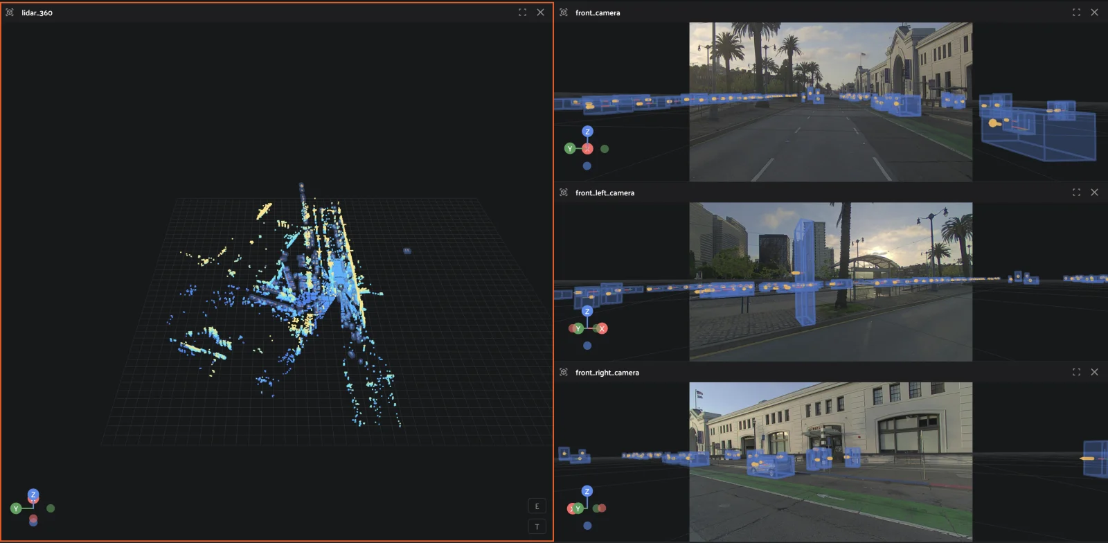
To add another 3D tile, open the  Layout menu and choose
Add tile → 3D. Several 3D tiles can show different views of the same
frame. Keyboard shortcuts and the annotation toolbar belong to the focused 3D
tile, or to the first one when none has focus.
Note
This 3D tile is not the 3D tile of multimodal datasets, which plays MCAP and LeRobot recordings.
Tile settings#
Each 3D tile has a Tile tab in the sidebar. Its sections fold, and each shows a one-line summary when folded.
Source chooses which point cloud slices to show. It appears when the group has two or more point cloud slices, applies to every 3D tile, and keeps at least one slice selected.
Display turns scene aids on and off:
Grid: on by default
Background: shown when the scene has a background
Cameras: the camera frustums, shown when the scene has cameras
Points: on by default, off in camera views
Image: the camera image, in camera views only
Points styles the point cloud:
Shade by: Height (default), RGB when the points have color, any scalar channel by name, or Custom color
Colormap: Viridis by default. Also Cool-warm, Grayscale, Inferno, Jet, Magma, Plasma, Turbo and Cyan to yellow.
Threshold: for scalar channels, hides points outside a value range
Point size: 0.1 to 20, default 2
Attenuate by distance: shrinks far points, off by default
Labels styles 3D labels:
Polyline width: shown when the dataset has polyline fields
Cuboid line width: 1 to 20, default 3
Cuboid headings: draws the heading arrow on every cuboid, off by default
Label opacity comes from Label opacity in the color scheme.
Note
The Points and Labels settings are saved in your browser and apply to every 3D tile.
Dataset owners can set a default colormap per attribute; see Default colormaps per attribute.
Camera views#
The View picker in the Tile tab sets how the tile looks at the scene. Each tile remembers its view across samples, and saved layouts keep it. If a sample lacks the chosen camera, the tile falls back to Orbit.
Orbit is the default. Drag to rotate, Shift + drag or right-drag to pan, and scroll to zoom toward the pointer. The E and T buttons in the tile’s corner, or the E and T keys, jump to an ego view and a top view. Choose Orbit again to reset the camera.
Cuboid top, Cuboid bottom, Cuboid right, Cuboid left, Cuboid front and Cuboid back lock the camera to the selected cuboid and follow it as the scene plays. Points outside the cuboid, plus a 1.5 m margin, are hidden, so the object stands out. With several cuboids selected, the view frames all of them. With none selected, it frames the point clouds once.
One entry per calibrated camera, named after its slice, locks the tile’s camera to that camera’s position and draws its image behind the scene. The tile is still the full 3D editor: you draw, select and edit cuboids on the image exactly as in Orbit. Points start hidden; turn them on in Display.
Note
A 3D tile set to a camera view looks much like a 2D tile showing the same camera slice, but they do different jobs. Use a 3D tile with a camera view to annotate cuboids and 3D polylines on the LiDAR slice. Use a 2D tile of a camera slice to annotate 2D labels, such as bounding boxes, on that image. 3D annotation needs no 2D tiles.
In camera and cuboid views, scrolling is a lens zoom from 1× to 8×. In camera views it zooms toward the pointer and dragging pans. Changing the view resets the zoom.
Double-click a cuboid to move the camera so that cuboid’s track is in view.
Classification chips#
Classifications and regressions on a 3D sample appear as chips in the tile’s top-left corner. Click a chip to select its label; Shift + click adds or removes it from the selection.
How to: Annotate in 3D#
Getting started#
Switch to the Annotate tab. The sidebar lists the cuboid and polyline tools of your annotation schema, and a toolbar appears on the 3D tile when a tool is active. Pick the class for new cuboids in New cuboid class.
You can edit a field only once it’s in the dataset’s annotation schema. Loading cuboids doesn’t add their field: to edit them, add the field in the Schema Manager, from the Annotate tab. Until then you can select them but not change them.
Edits save automatically. Use Undo (Cmd+Z) and Redo (Cmd+Shift+Z); on Windows and Linux, use Ctrl instead of Cmd. See Saving and Reverting Changes.
To annotate as part of a team, with batches, review and assigned tasks, see Projects.
Annotation plane#
A click in a 3D scene needs a depth. By default it lands on the ground under the pointer, at the height of the LiDAR points there. Clicks pass through unselected cuboids to the ground below.
To draw on a slope or a raised surface, turn on  Annotation plane. A plane appears, level at the scene’s origin. Choose
Move plane to drag it with arrows, or Tilt plane to turn it with rings,
for example onto a ramp. While the plane shows, new cuboids sit on it, with
their up axis along the plane’s normal. Your browser remembers the plane’s
position for each dataset, but the plane starts hidden every time.
How to: Annotate cuboids#
Drawing a cuboid#
Choose  Draw (D), then click three times on the
ground:
One corner of the object.
The end of its long side. This sets the length and the heading. You can drag instead of clicking.
Its width.
The height fits the points inside the footprint. Right-click or press Esc before the third click to cancel.
The video at the top of this page shows a cuboid drawn in a camera view, then moved and resized.
Tip
Draw from the top view (T). The footprint is easiest to see from above.
Selecting and framing#
Click a cuboid to select it. Press Z or choose  Frame the selected cuboids to zoom to the selection; with nothing
selected, Z frames the whole scene. Press Esc to clear the
selection.
Moving, rotating and resizing#
With one cuboid selected:
 Move (G): drag an arrow or a plane handle. The
handles follow the cuboid’s own axes.
 Rotate (R): drag a ring to turn the cuboid
about one of its three axes, so pitch and roll as well as heading.
 Resize (S): pull one of the six face handles.
That face moves and the opposite face stays put.
The camera holds still while you drag a handle.
Annotating across views#
All 3D tiles show the same cuboids, so you can work in several views at once. A typical layout:
an Orbit tile for the overview and for drawing
two or three camera tiles to check each cuboid against the images
a Cuboid top tile to fine-tune the footprint of the selected cuboid
Draw, select, move, rotate and resize in whichever tile shows the object best. Selection is shared, and while you drag in one tile, every other tile follows. A cuboid that looks right from above but sits off the car in the front camera is easy to catch this way. The video at the top of this page shows this layout at work.
Heading#
A cuboid’s heading arrow marks its front. The selected cuboid always shows it; turn on Cuboid headings in the Tile tab to show it on every cuboid.
If a cuboid faces the wrong way, drag its heading arrow onto the dot of the face that should be the front. The box stays where it is; only its front changes. On a track, every frame of the track changes in one undo step. Release on the same face, or press Esc, to cancel.
In the clip, Cuboid headings is turned on, then the arrow is dragged to the dot on the rear face:
Position, dimensions and rotation#
The Edit panel in the sidebar shows the selected cuboid’s Position, Dimensions and Rotation (X, Y and Z each). Rotation is shown in degrees and stored in radians. Type a value to change it. On a track, editing a value makes that frame a keyframe.
Attributes and fields#
The Edit panel also shows the attributes defined in the Schema Manager. To move a cuboid to another label field, pick the field in Label field. The whole track moves, keeps its identity, and the move is one undo step.
Deleting#
Delete or Backspace removes the selected cuboids from the current frame only. To remove a whole track, use Delete track on the timeline.
How to: Annotate tracks#
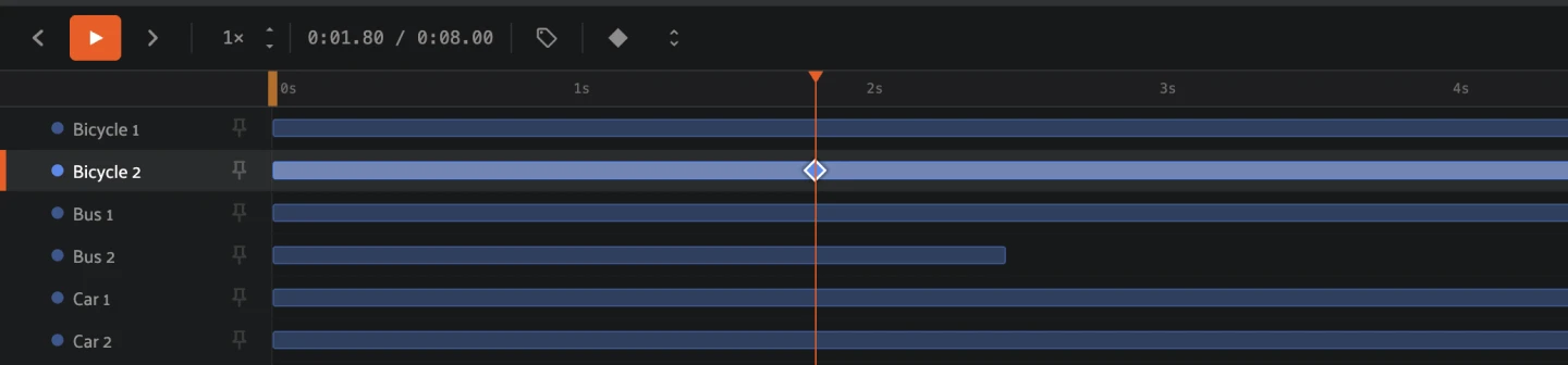
3D tracks work like video object tracks: a row per track on the timeline, keyframes as diamonds, and the same split, merge and drag operations. This section covers what differs in 3D: World and Ego frames, drawing onto a selected track, and how merging re-interpolates. A track’s cuboids share an Instance.
Tracks on the timeline#
Each track is a row on the timeline, named by class and number, such as Car 12. The bar shows the frames where the track exists, and diamonds mark its keyframes.
Selecting a cuboid highlights its row and scrolls the timeline to it. Clicking a row selects the track.
Creating a track: World and Ego#
With no track selected, draw a cuboid. The App starts a new track and fills the next 3 seconds of frames after it, stopping at the end of the scene.
The New frames setting decides how those filled frames move. It appears in the tile toolbar when the tile plays a scene. Pick it before you draw.
 World (the default) keeps the filled frames fixed on the
ground. Use it for parked cars, signs and anything else that stands still
while the vehicle drives. Here, a cuboid drawn on a parked car stays on it as
the vehicle passes:
 Ego moves the filled frames along with the vehicle. Use it
for traffic driving alongside. Here, a cuboid drawn on a car in the next lane
rides along with it:
The fill is a starting point; correct it with keyframes. Switching the setting never changes existing frames. It stays set while you move between samples and resets to World when you reload the page.
Keyframes and interpolation#
Moving, rotating, resizing or typing a pose value makes the current frame a
keyframe, and the App re-interpolates the frames between it and its neighbors.
When every frame has an ego_pose, interpolation happens in world
coordinates, so an object between two keyframes moves smoothly on the ground
even while the vehicle turns.
 Mark Keyframe (K) turns the current frame
into a keyframe, or back into an interpolated frame. Removing a keyframe
re-interpolates across the gap. A track’s only keyframe can’t be removed.
[ and ] jump to the previous and next keyframe of the selected tracks, or of all tracks when none is selected.
To follow an object past the fill, drag the end of the track’s bar to extend it. Then step through the track and move the cuboid back onto the object wherever it drifts. Each correction adds a keyframe:
Tip
Instead of adjusting a cuboid, you can draw a new one on the object, which is often faster. See Adding a keyframe by drawing.
Adding a keyframe by drawing#
Draw does one of two things, depending on the selection:
A cuboid is selected: the drawing becomes a new keyframe of that cuboid’s track, at the current frame. The tooltip reads “Draw a keyframe on Car 12”.
Nothing is selected: the drawing starts a new track. The tooltip reads “Draw a cuboid”.
When drawing onto a track:
It works anywhere on the timeline, including past the track’s end; the toolbar stays available on frames where the track has no cuboid.
The new cuboid takes its size, class and attributes from the track’s nearest keyframe. Draw sets only position and heading; resize with S afterwards if needed.
Frames between the new keyframe and the rest of the track are filled in.
To start a new track instead, press Esc to clear the selection, then draw.
Merging and splitting tracks#
When one object ended up as two tracks, right-click one track’s bar and choose Merge into another track of the same class and field. The tracks become one:
Where both tracks have a frame, the target track’s frame wins, except that a keyframe always beats an interpolated frame.
Only the overlapping frames are re-interpolated. A gap between the tracks stays empty.
To cut a track in two, choose Split at playhead from the bar’s menu, or
 Split in the toolbar. Both sides of the cut become
keyframes. Merging and splitting are each one undo step.
Other timeline operations#
These work as they do for video.
Drag to retime. Drag a track’s bar to shift it, or drag either end to extend or trim it.
Track menu. Right-click a track’s bar for Move to start, Move to end, Shrink window to fit, Merge into, Split at playhead, Delete track and Delete current frame.
Pin. Pin a track to keep its row at the top of the timeline.
Loop. Right-click the ruler to loop playback over a range.
How to: Annotate 3D polylines#
Choose  New Polyline (P) and click each
vertex. Double-click, press Enter or right-click to finish.
The polyline toolbar:
 New Segment: adds a segment to the selected
polyline
- Move (G): moves the selected vertex, or the
whole polyline
 Edit Segments: click an edge of the selected
polyline to insert a vertex
 Snap Close: closes every new polyline into a loop
Delete or Backspace deletes the selected vertex.
Polyline tracks#
In a scene, polylines form tracks just as cuboids do: each track gets a row on the timeline, a new polyline fills the next 3 seconds following New frames (World or Ego), and frames between keyframes are interpolated. Mark Keyframe (K), Split and Merge work the same way. One difference: drawing a polyline always starts a new track, even when a track is selected.
Segments, closed and filled#
One 3D polyline can hold several separate segments that
share a label and its attributes. In the SDK, points3d is a list of
segments, each a list of [x, y, z] points in scene coordinates:
1# Two segments of one polyline, for example two dashes of a lane marking
2points3d = [[[-5, -99, -2], [-8, 99, -2]], [[4, -99, -2], [1, 99, -2]]]
A polyline also has two display attributes. closed joins the last vertex back to the first, and filled shades the enclosed area.
Keyboard shortcuts#
Press ? in the App to see every keyboard shortcut. The 3D tile, Timeline and Annotate 3D tabs list the keys for the tools on this page.
Configuring the 3D viewer#
Set defaults for every 3D tile under the plugins.3d key of your
App config, or for one dataset in its
App config. Dataset settings override the global
ones.
1dataset.app_config.plugins["3d"] = {
2    "defaultUp": [0, 0, 1],
3    "defaultCameraPosition": {"x": 0, "y": 0, "z": 100},
4    "pointCloud": {"minZ": -2},
5}
6dataset.save()
defaultUp: the scene’s up direction. A.fo3dscene’s own up direction wins.defaultCameraPosition: where the Orbit camera starts, as[x, y, z]or{"x": …, "y": …, "z": …}. A.fo3dscene’s own camera wins.pointCloud.minZ: the height where Height shading starts its colormap. Points below it are still shown.
Default colormaps per attribute#
To give a point cloud attribute a default colormap, add a colorscale for it to
the dataset’s color scheme, with the path
::fo3d::pcd::<attribute>. When you shade by that attribute, the Colormap
list shows App config and uses it by default. Height shading keeps the
tile’s own colormap.
 1import fiftyone as fo
 2
 3dataset = fo.load_dataset("my-drives")
 4dataset.app_config.color_scheme = fo.ColorScheme(
 5    colorscales=[
 6        {"path": "::fo3d::pcd::intensity", "name": "viridis"},
 7        {
 8            "path": "::fo3d::pcd::lidar_id",
 9            "list": [
10                {"value": 0, "color": "rgb(0, 0, 255)"},
11                {"value": 1, "color": "rgb(0, 255, 255)"},
12            ],
13        },
14    ],
15)
16dataset.save()