FiftyOne Multimodal

FiftyOne provides native support for multimodal datasets, which represent rich, time-synchronized sensor recordings such as robotics and autonomous vehicle logs stored in the MCAP container format and episodic robot learning data in the LeRobot dataset format.

A single multimodal sample can contain many concurrent data streams — camera images, LIDAR point clouds, IMU readings, GPS fixes, coordinate frame transforms, robot states and actions, diagnostics, and more — and FiftyOne lets you visualize, play back, tag, and query all of them in lockstep.

Note

Multimodal visualization is available to all FiftyOne users. With FiftyOne Enterprise you can additionally index your MCAP data (currently in beta) into columnar tables that power scalable search, filtering, and event mining across your entire fleet of recordings, and compute segment embeddings (also in beta) to visually explore, find similar moments in, and semantically search your recordings.

Overview

A multimodal dataset is a FiftyOne dataset whose media type is "multimodal" and whose samples are episodes: recordings that bundle many concurrent, timestamped data streams. FiftyOne supports two multimodal recording formats:

• MCAP: self-describing container files for heterogeneous robotics data, typically produced by ROS or Foxglove tooling

• LeRobot: episodic robot learning datasets containing camera streams and state/action trajectories

The same key concepts apply to both formats:

• Episodes: each sample in a multimodal dataset is an episode — one recording

• Streams: each data stream in the recording — an MCAP channel (topic), or a LeRobot feature — can be bound to one or more tiles in the viewer

• Time tracks: every message carries timing information (timestamps for MCAP; frame times for LeRobot) that drives synchronized playback across all tiles

When you open a multimodal sample in the App, FiftyOne reads the source data directly via efficient byte-range reads — no server-side conversion is required — discovers its streams, decodes the data it knows how to interpret, and renders it in a configurable, tiled viewer with a shared playback clock.

MCAP datasets

MCAP is a self-describing container format for heterogeneous, timestamped robotics data that stores messages organized into channels (topics), each with an associated schema describing how to decode its payloads.

When you add samples whose filepaths end in .mcap, the dataset’s media type is automatically inferred as "multimodal":

import fiftyone as fo

dataset = fo.Dataset("robot-teleop-episodes")
dataset.add_samples(
    [
        fo.Sample(filepath="/path/to/episode-0001.mcap"),
        fo.Sample(filepath="/path/to/episode-0002.mcap"),
    ]
)

print(dataset.media_type)  # multimodal

LeRobot datasets

LeRobot is a widely used format for episodic robot learning data. FiftyOne natively supports LeRobot v3 datasets: import one via the fiftyone.types.LeRobotDataset dataset type, which creates one sample per logical episode:

import fiftyone as fo

dataset = fo.Dataset.from_dir(
    dataset_dir="/path/to/lerobot-dataset",
    dataset_type=fo.types.LeRobotDataset,
    name="robot-learning-episodes",
)

print(dataset.media_type)  # multimodal

Unlike MCAP samples, LeRobot samples do not point to a single file. Each sample is a lightweight episode reference into the source dataset — its meta/info.json, episode metadata, Parquet frame data, and MP4 videos are read on demand — and each sample is automatically populated with episode-level fields (episode_index, task, tasks, length, duration, robot_type, and fps) that you can filter and query like any other FiftyOne fields. Imports are fast because only the source’s metadata is read at import time.

A dataset can reference episodes from multiple LeRobot sources: use add_dir() to add additional sources to an existing dataset, and each source is recorded on the dataset as it arrives:

dataset.add_dir(
    dataset_dir="/path/to/another-lerobot-dataset",
    dataset_type=fo.types.LeRobotDataset,
)

Because an episode only resolves through a source its dataset records, always build LeRobot datasets from directories as shown above — adding individual samples cannot introduce a new source.

You can also export any collection of LeRobot samples back to a self-contained LeRobot v3 dataset.

Note

LeRobot support requires pyarrow>=10.0.0 and currently supports LeRobot v3 datasets. Because samples reference the source dataset rather than copying it, re-import your dataset if the underlying LeRobot source is modified or moved.

Grid previews

In the App’s sample grid, each multimodal sample displays a preview rendered from one of its streams, and you can use the stream selector to choose which stream is used for grid previews. Camera streams are preferred by default, and your stream selection persists across episodes.

In FiftyOne Enterprise, grids over indexed MCAP datasets load instantly from automatic thumbnails generated during indexing.

Tiles

Multimodal samples open in a configurable, mosaic-style viewer composed of tiles. You can add, remove, resize, and rearrange tiles, and bind each tile to any compatible stream in the recording. All tiles share a common playback clock, so scrubbing the timeline updates every tile in sync.

The same viewer is used for both MCAP and LeRobot episodes, but the set of available tile types depends on the recording format and the streams it actually contains — a tile type is only offered when the episode has at least one stream it can display:

Tile	MCAP	LeRobot
Image	✓	✓
Audio	✓
3D	✓
Map	✓
Plot	✓	✓
Message	✓	✓
Logs	✓
Transforms	✓
State & Action		✓

Image tile

Image tiles render camera streams. For MCAP recordings, this includes raw and compressed images from ROS and Foxglove schemas as well as compressed video streams (currently H.264); for LeRobot episodes, this includes both video features (H.264 and AV1) and image features whose frames are stored inline in the episode’s Parquet data.

For MCAP recordings, image annotations (e.g. foxglove.ImageAnnotations) can be overlaid on their corresponding camera stream, and when camera calibration data is available, hovering over an image tile highlights that camera’s frustum in the 3D tile.

Audio tile

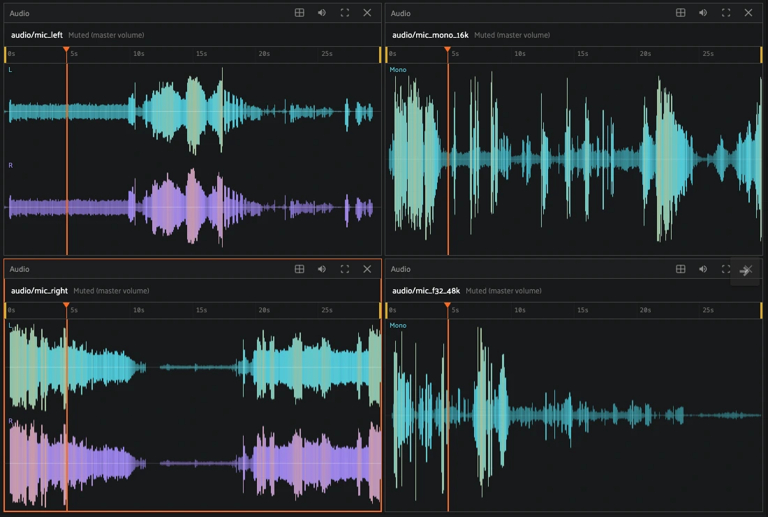
The audio tile renders waveforms for the audio streams in MCAP recordings — foxglove.RawAudio (8/16/32-bit integer and 32-bit float PCM) and foxglove.CompressedAudio (Opus) — which play back in sync with the shared clock. An open audio tile isn’t required to hear a recording: any recording with audio streams gets volume and per-track mute controls in the playback bar, and the tile adds the waveform view for a selected stream.

3D tile

The 3D tile renders the spatial content of your MCAP recording in a shared world frame: point clouds (with configurable colormaps and color-by fields such as intensity), laser scans, occupancy grids, scene-update primitives, pose trajectories, and camera frustums. Coordinate frame transforms from the recording are used to place everything correctly, and you can select the reference frame, track a moving frame with the camera, measure distances, and inspect points via hover tooltips.

Map tile

The map tile plots GNSS location streams (e.g. foxglove.LocationFix or sensor_msgs/msg/NavSatFix) as tracks on an interactive map. The current position follows the playback clock, and you can hover to inspect points along the track and measure distances between locations.

Plot tile

Plot tiles chart numeric series extracted from any stream and field path in the recording — IMU rates, vehicle speed, steering angle, diagnostics values, robot state and action dimensions, etc. — over the full duration of the recording. A playhead marks the current playback position, and clicking anywhere in the plot seeks the shared clock to that time.

Message tile

The message tile is the escape hatch for any stream, decoded or not: it displays the most recent record on a selected stream at the current playhead — an MCAP message, or a LeRobot episode row — as a collapsible record tree, so you can inspect exact field values as you scrub through the recording.

State & Action tile

The State & Action tile is available for LeRobot episodes and provides exact single-row inspection of the episode’s observation.state and action features. At any playhead position it shows the state and action vectors from the corresponding episode row — with per-dimension names when the dataset declares them — and previous/next controls step an exact row cursor while seeking the camera tiles to the row’s timestamp. Any individual dimension can be added to a Plot tile with one click to chart it over the episode.

The tile’s settings let you choose the value scale (raw values, z-scores, or quantiles, derived from the dataset’s declared statistics in meta/stats.json) and the marker range used to contextualize each value (this episode’s observed min–max, or the dataset’s declared range with a q01–q99 band and out-of-range flagging).

Logs tile

The logs tile is a console view for log topics in MCAP recordings (foxglove.Log, rcl_interfaces/msg/Log, rosgraph_msgs/Log). Log entries scroll in sync with the playback clock, and you can pause following to scan the history or seek the recording to an entry of interest.

Transforms tile

The transforms tile is a diagnostic view of an MCAP recording’s coordinate frame topology. It renders the frame graph — every coordinate frame and the transform streams connecting them — and flags structural issues in the recording, such as cycles, frames with multiple parents, self-edges, frame name mismatches, and disconnected components whose streams cannot be co-registered in the 3D tile. You can search for frames, select frames and edges to inspect their details, and extend the analysis to cover more of the recording on demand.

Configuring tiles

To add a new tile to the viewer, click the Add tile button (the grid icon) in the viewer’s header and choose from the tile types available for the current episode. The same menu also offers Auto Layout, which automatically arranges your tiles.

The left sidebar of the viewer is where you configure what each tile is showing. It contains the following tabs:

• Scene: settings that apply to the whole recording:

  • Playback: choose how signals behave between recorded samples — Smooth interpolates continuous signals (transforms and 2D/3D label geometry) for fluid playback, while As recorded never synthesizes values and holds each signal at its latest recorded sample

  • Advanced timing: fine-grained control over how messages are matched to the playback clock

• Topics (MCAP) / Streams (LeRobot): a searchable inventory of every stream in the recording, grouped by category — Sensors, Annotations & Planning, Transforms & Poses, Diagnostics, Telemetry, and Custom/Unknown for MCAP recordings; Observations, Actions, Instructions, and Custom for LeRobot episodes. Each stream shows how it can be visualized, and you can open a stream directly in a compatible tile from here

• Tile settings: when you focus a tile, a tab named for that tile appears with its specific options — for example, which streams and overlays an image tile displays, the 3D tile’s colormaps and camera behavior, the topic/field series charted by a plot tile, or the topic shown in a message tile

Inspecting objects

For MCAP recordings, the right sidebar of the viewer is an inspector for objects in the scene. Click any object in any tile — a 3D box in the 3D tile or an annotation in an image tile — to view its details:

• For 3D scene objects: the object’s label, entity ID, topic, coordinate frame, and any metadata attached to the object

• For image annotations: the object’s label, primitive kind, topic, and exact geometry

Any fields not covered by the structured view are shown as raw JSON. Press Esc or click Clear selection to clear the current selection.

For LeRobot episodes, which have no pickable scene objects, the right sidebar instead shows a Statistics tab summarizing the episode’s state and action data per dimension: the dataset’s declared statistics (from meta/stats.json), this episode’s computed statistics — including seekable extremes that jump the playhead to where a min/max occurred — recorded cadence, out-of-declared-range counts, and action-vs-state tracking error.

Timeline tracks

Beneath the playback timeline, the viewer displays tracks: rows of time-anchored context that scrub in sync with the recording. Tracks are organized into sections that only appear when they have content:

• Temporal tags: the temporal tags on the current sample, which you can create directly on the timeline

• Events: intervals for derived events computed by MCAP indexing, e.g. “high steering” or “pedestrian while moving”. Event tracks only appear when the recording has derived events

• Labels: annotations over time, one track per annotation topic. Label tracks only appear while annotations are currently visible in one of your tiles

• Embedding windows: the time spans of any segment embeddings currently selected in the Embeddings panel

Note

Event, label, and embedding window tracks are only available in FiftyOne Enterprise; event tracks additionally require MCAP indexing and embedding window tracks require segment embeddings.

MCAP Explorer

FiftyOne also includes a standalone MCAP Explorer panel that lets you open an arbitrary local .mcap file (via drag-and-drop or file browser) or a remote URL without creating a dataset first. Local files stay in your browser session and are read directly — nothing is uploaded.

Temporal tags

Multimodal samples span long time ranges, so FiftyOne supports temporal tags: tags attached to a time interval within a sample rather than to the whole sample. Temporal tags are ideal for marking events of interest — interventions, near-misses, sensor dropouts, interesting maneuvers.

You can create temporal tags interactively in the App, or programmatically via the SDK.

Tagging in the App

To create a temporal tag in the App, Shift + click and drag along the playback timeline to select the interval of interest, then enter the tag. Existing tags appear on the timeline, where you can review and delete them.

Tagging via the SDK

You can create and read temporal tags programmatically:

import fiftyone as fo
import fiftyone.core.tags as fota

dataset = fo.load_dataset("robot-teleop-episodes")
sample = dataset.first()

# Tag the interval [start, end) on a sample, expressed in nanoseconds
# elapsed since the start of the recording
dataset.temporal_tags.add(
    fota.TemporalTag(
        sample.id,
        start=4_000_000_000,  # 4s, inclusive
        end=6_000_000_000,  # 6s, exclusive
        tag="gripper closed",
    )
)

# Retrieve the collection's temporal tags
print(dataset.temporal_tags)

You can also filter your dataset to samples whose temporal tags match given criteria:

# Samples containing at least one "gripper closed" temporal tag
view = dataset.match_temporal_tags(tags="gripper closed")

Supported schemas

The data that FiftyOne can decode and visualize depends on the recording format. In both cases, any stream that is not recognized remains fully accessible via the Message tile, so you can always inspect your data even before a dedicated decoder exists.

MCAP

FiftyOne ships with built-in decoders for visualizing the MCAP message schemas below in the App.

ROS

Both ROS 1 and ROS 2 messages are supported for the following schemas, listed here in their ROS 2 form (the corresponding ROS 1 schemas are also supported):

Schema	Description
sensor_msgs/msg/Image	Raw camera images, including common pixel encodings (rgb8, bgr8, rgba8, bgra8, mono8, mono16), YUV formats, depth encodings (16uc1, 32fc1), and Bayer-patterned formats
sensor_msgs/msg/CompressedImage	Compressed (e.g. JPEG/PNG) camera images
sensor_msgs/msg/CameraInfo	Camera intrinsics and distortion parameters, rendered as camera frustums in the 3D tile
sensor_msgs/msg/PointCloud2	LIDAR and other point clouds, with support for per-point scalar fields such as intensity
sensor_msgs/msg/LaserScan	Planar laser range scans
sensor_msgs/msg/NavSatFix	GNSS position fixes, rendered in the map tile
nav_msgs/msg/Odometry	Odometry poses with velocity/acceleration kinematics
nav_msgs/msg/Path	Pose sequences such as planned or traveled paths
nav_msgs/msg/OccupancyGrid	Occupancy grids, rendered as textured planes in 3D
geometry_msgs/msg/PoseStamped	Single timestamped poses
geometry_msgs/msg/PoseArray	Batches of poses
geometry_msgs/msg/TransformStamped	Single coordinate frame transforms
tf2_msgs/msg/TFMessage	Coordinate frame transforms that define the scene’s frame graph
visualization_msgs/msg/Marker / visualization_msgs/msg/MarkerArray	Scene markers (cubes, spheres, lines, text, meshes) rendered in the 3D tile
vision_msgs/msg/Detection2DArray	2D detections overlaid on camera images
vision_msgs/msg/Detection3DArray	3D detections rendered in the 3D tile
diagnostic_msgs/msg/DiagnosticArray	Diagnostics status arrays
rcl_interfaces/msg/Log	Log messages (rosgraph_msgs/Log in ROS 1), shown in the logs tile

Foxglove

All of the core Foxglove schemas are supported, in both their protobuf and ROS (CDR) encodings:

Schema	Description
foxglove.RawImage	Raw camera images
foxglove.CompressedImage	Compressed camera images
foxglove.CompressedVideo	Compressed video streams (currently H.264)
foxglove.RawAudio	Raw PCM audio streams (8/16/32-bit integer and 32-bit float), rendered in the audio tile
foxglove.CompressedAudio	Compressed audio streams (currently Opus), rendered in the audio tile
foxglove.ImageAnnotations	2D annotations (points, circles, text) overlaid on camera images
foxglove.CameraCalibration	Camera intrinsics and distortion, rendered as camera frustums
foxglove.PointCloud	Point clouds with per-field data
foxglove.LaserScan	Planar laser range scans
foxglove.Grid	2D data grids (e.g. occupancy/cost maps), rendered as textured planes in 3D
foxglove.SceneUpdate	Scene-graph primitives (arrows, cubes, spheres, lines, text, models)
foxglove.FrameTransform	A single coordinate frame transform
foxglove.FrameTransforms	A batch of coordinate frame transforms
foxglove.PoseInFrame	SE(3) poses (translation + quaternion)
foxglove.LocationFix	GNSS position fixes (latitude/longitude/altitude), rendered in the map tile
foxglove.Log	Log messages, shown in the logs tile

JSON

Channels containing JSON-encoded messages are supported for the following schemas:

Schema	Description
Pose	JSON-encoded pose/odometry data
JSON-encoded ROS schemas	JSON-encoded versions of the ROS schemas above (e.g. sensor_msgs/PointCloud2, nav_msgs/Odometry) are decoded just like their binary counterparts

LeRobot

LeRobot datasets are self-describing: FiftyOne decodes an episode from the features declared in the dataset’s meta/info.json, and each feature becomes a stream in the viewer:

Feature	Description
video features	MP4 camera streams, rendered in image tiles. H.264 and AV1 codecs are currently supported in the App
image features	Camera frames stored inline in the episode’s Parquet data, rendered in image tiles
Numeric features (float*, int*, uint*, bool)	Per-dimension numeric series — including observation.state and action — available in plot tiles and the State & Action tile. When the dataset declares dimension names (flat, nested, or axis-dict style), they are used to name the individual series
Text features (task/instruction/prompt/language)	Natural language task instructions

Streams are automatically categorized as Observations (observation.*), Actions, Instructions, or Custom, and standard bookkeeping columns (timestamp, frame_index, episode_index, index, task_index) are consumed automatically rather than surfaced as streams. When present, per-dimension statistics from meta/stats.json and task metadata from meta/tasks.parquet are also used throughout the viewer.

Exporting multimodal datasets

Multimodal datasets can be exported via export() like any other FiftyOne dataset. There are two main paths: exporting in FiftyOneDataset format for full-fidelity round trips between FiftyOne installations, and exporting curated episodes to a new LeRobot dataset for consumption by robot learning tooling.

FiftyOneDataset format

Exporting in FiftyOneDataset format round-trips a multimodal dataset with full fidelity — samples, fields, views, and temporal tags included:

import fiftyone as fo

dataset = fo.load_dataset("robot-teleop-episodes")

dataset.export(
    export_dir="/path/for/export",
    dataset_type=fo.types.FiftyOneDataset,
)

dataset2 = fo.Dataset.from_dir(
    dataset_dir="/path/for/export",
    dataset_type=fo.types.FiftyOneDataset,
)

The export_media behavior depends on how the collection’s media is stored:

• MCAP datasets: samples are ordinary files, so the standard modes apply — pass export_media=True to copy the .mcap files into the export, or export_media=False to export only sample records that point to the existing files

• LeRobot datasets: samples are episode references, so export_media=True materializes every referenced asset into a self-contained export (assets shared by multiple episodes are only copied once), while export_media=False writes a thin export containing the sample records and their source bindings. A thin export does not copy the LeRobot source itself, so the source must remain available and unmodified wherever the export is later imported

Exporting to LeRobot format

Any collection of LeRobot episodes from a single source — an entire dataset, or a view containing the episodes you’ve curated — can be exported as a new, self-contained LeRobot v3 dataset that any LeRobot-compatible tooling can consume:

import fiftyone as fo

dataset = fo.load_dataset("robot-learning-episodes")

# Curate the episodes you care about
view = dataset.match_temporal_tags(tags="gripper closed")

# Export them as a new LeRobot v3 dataset
view.export(
    export_dir="/path/for/lerobot-export",
    dataset_type=fo.types.LeRobotDataset,
)

The exported dataset contains only the selected episodes, rewritten as a valid standalone LeRobot dataset: episodes are renumbered contiguously, task and global frame indexes are rebuilt, and the relevant videos and Parquet frame data are copied over. Every export is validated after writing — including against the official lerobot reader, when it is installed.

Note the following requirements:

• All episodes in the collection must come from the same source LeRobot dataset

• LeRobot exports are always self-contained: export_media=True is the only supported mode. To export thin references instead, use the FiftyOneDataset format described above

Indexing MCAP data BETA

Available in: Enterprise

Introduced in FiftyOne Enterprise 2.22.0

Schedule a demo to get started with FiftyOne Enterprise

Note

MCAP indexing is only available in FiftyOne Enterprise. It is currently in beta and is disabled by default; contact your deployment administrator or Voxel51 support to enable the feature for your deployment.

MCAP files are optimized for recording and playback, not for analytical queries. Questions like “find every episode where a pedestrian was visible while the vehicle was moving faster than 5 m/s” would otherwise require scanning and decoding every file in your fleet.

FiftyOne Enterprise solves this by indexing your MCAP data: a projection pipeline reads each recording once, decodes the channels you declare, and writes the results to columnar Parquet tables (managed via Apache Iceberg) called projections. These tables power fast, scalable filtering, aggregation, and event search across your entire dataset — in the App’s grid, sidebar, and query interfaces — without ever re-reading the source MCAPs.

The indexing pipeline maintains its own decoder registry, which currently covers the core ROS 2, Foxglove, and JSON message schemas (e.g. images, point clouds, IMU readings, poses, diagnostics, and image annotations).

You control exactly what gets indexed by authoring a projection manifest. Four kinds (grains) of projections are supported:

• labels: per-message rows extracted from annotation streams, e.g. the text and geometry of every image annotation

• signals: numeric time series sampled from message fields, e.g. vehicle speed, steering angle, or IMU rates, with configurable sampling strategies

• events: derived time intervals computed from other projections using expressions, e.g. “windows of high steering lasting at least 500ms”

• summaries: per-episode scalar rollups, e.g. the max speed or whether any pedestrian was observed

Indexing runs as delegated operations that are automatically scheduled and orchestrated across your deployment’s compute. Projection tables can be written to local storage or directly to cloud buckets (s3://, gs://, az://).

Enabling indexing

Any dataset containing MCAP samples is automatically registered as a multimodal dataset. To index it, configure it with a projection manifest and enable projections:

import fiftyone as fo

dataset = fo.Dataset("robot-teleop-episodes")
dataset.add_samples(
    [
        fo.Sample(filepath="/path/to/episode-0001.mcap"),
        fo.Sample(filepath="/path/to/episode-0002.mcap"),
    ]
)

# Configure the dataset with your manifest and enable indexing
with open("/path/to/manifest.yaml", "r") as f:
    dataset.projections.enable(f.read())

Indexing is then scheduled and executed automatically. You can check on its progress, disable it, or retry a stuck run at any time:

# The active run's status, including per-sample progress
print(dataset.projections.get_projection().status())

# Disable indexing, abandoning any active run
dataset.projections.disable()

# Reset a run that was interrupted (e.g. its worker crashed) so that it
# is automatically requeued
dataset.projections.retry()

Authoring manifests

A projection manifest is a YAML document that tells the indexing system what data to extract from your MCAP files and how to organize it. A manifest has four top-level keys:

sink: ...                     # where projection tables are written
channel_bindings: ...         # which MCAP channels to read
channel_binding_repeats: ...  # templated bindings for repeated sensors
projections: ...              # the tables to build from those channels

Sink

The sink section declares where projection tables are written. The location may be a local path or a cloud bucket URI:

sink:
  type: iceberg  # the default
  location: s3://my-bucket/projections

Channel bindings

A channel binding selects a channel from your MCAP files and gives it a stable id that projections can reference. Channels are selected by match-ing on their topic, schema name, and encoding, and can optionally be filtered with a where expression:

channel_bindings:
  - id: diagnostics_steering_angle
    match: { topic: /diagnostics, schema_name: Diagnostics, encoding: json }
    where: 'name == "Steering Angle"'
    timestamp_source:
      candidates:
        - mcap: MCAP_MESSAGE_TIME_LOG_TIME

Each binding supports the following fields:

• id: a unique identifier for the binding

• match: the channel selector, with keys topic, schema_name, and encoding

• where (optional): an expression that filters messages within the channel, e.g. when multiple logical signals share a single topic

• timestamp_source: an ordered list of candidates declaring where each message’s timestamp comes from. Each candidate is either:

  • decoded: { path: <field.path> }: a timestamp field decoded from the message payload

  • mcap: MCAP_MESSAGE_TIME_LOG_TIME or mcap: MCAP_MESSAGE_TIME_PUBLISH_TIME: the MCAP record’s log or publish time

Channel binding repeats

Multi-sensor rigs typically have many channels with identical structure (e.g. six cameras). Rather than duplicating bindings, use channel_binding_repeats to declare a template that is expanded once per sensor using {{var}} substitution:

channel_binding_repeats:
  - var: camera
    values:
      - { stream_id: cam_front, topic: CAM_FRONT }
      - { stream_id: cam_back, topic: CAM_BACK }
    templates:
      - id: "{{camera.stream_id}}_annotations"
        match:
          {
            topic: "/{{camera.topic}}/annotations",
            schema_name: foxglove.ImageAnnotations,
            encoding: protobuf,
          }
        timestamp_source:
          candidates:
            - decoded: { path: timestamp }
            - mcap: MCAP_MESSAGE_TIME_LOG_TIME

The example above expands into two channel bindings, cam_front_annotations and cam_back_annotations.

Projections

Each entry in projections declares one table. A projection names its sources — the channel bindings (or previously-defined projections) it reads from — and exactly one grain block (labels, signals, events, or summaries) describing the rows and columns to produce.

Labels extract one row per message (or per exploded array element) from annotation streams:

projections:
  - id: semantic_labels
    sources:
      - name: labels
        channel_bindings:
          - cam_front_annotations
          - cam_back_annotations
    labels:
      rows:
        for_each: labels
        explode: [texts, points]
        timestamp: labels.stream.timestamp
      columns:
        - { id: camera_id, value: labels.stream.id }
        - { id: label, value: labels.texts.text }
        - { id: image_points, value: labels.points.points }

Signals extract numeric time series. Columns may carry quantity and unit metadata, and values may be computed with expressions. The sampling block controls how the series is materialized:

projections:
  - id: imu_signals
    sources:
      - name: imu
        channel_bindings:
          - imu
    signals:
      rows:
        for_each: imu
        timestamp: imu.stream.timestamp
      sampling:
        strategy: SIGNAL_SAMPLING_STRATEGY_WINDOW
        window_ns: "50000000"
        aggregations:
          - SIGNAL_AGGREGATION_MEAN
          - SIGNAL_AGGREGATION_MAX
      clustering_keys: [timestamp_ns]
      columns:
        - {
            id: angular_velocity_x,
            value: imu.rotation_rate.x,
            quantity: angular_velocity,
            unit: rad/s,
          }

The available sampling strategies are:

• SIGNAL_SAMPLING_STRATEGY_NATIVE: one row per source message

• SIGNAL_SAMPLING_STRATEGY_WINDOW: aggregate values over fixed windows of window_ns nanoseconds, applying each of the requested aggregations (MEAN, MIN, MAX, FIRST, LAST, COUNT). Windowed aggregations produce suffixed columns, e.g. acceleration_norm_max

• SIGNAL_SAMPLING_STRATEGY_FIXED_RATE: resample at a fixed rate

• SIGNAL_SAMPLING_STRATEGY_ON_CHANGE: emit a row only when the value changes

Events derive time intervals from other projections. Each event definition has an occurrences block whose expr is an expression over source columns, with declared dependencies and tunable parameters:

projections:
  - id: derived_events
    sources:
      - name: vehicle_steering_signals
        projections:
          - vehicle_steering_signals
    events:
      definitions:
        - id: high_steering
          name: High steering
          description: Steering above threshold for a minimum duration.
          occurrences:
            expr: contiguous(abs(vehicle_steering_signals.steering_angle) > steering_high_threshold, steering_high_min_duration_ns)
            depends_on: [vehicle_steering_signals.steering_angle]
            parameters:
              steering_high_threshold:
                value: { number_value: 1.0 }
                quantity: steering_angle
              steering_high_min_duration_ns:
                value: { int64_value: "500000000" }
                quantity: time
                unit: ns

Summaries compute one scalar per episode, ideal for powering sidebar filters like “episodes containing a pedestrian”:

projections:
  - id: summaries
    sources:
      - name: semantic_labels
        projections:
          - semantic_labels
      - name: vehicle_speed_signals
        projections:
          - vehicle_speed_signals
    summaries:
      columns:
        - id: has_pedestrian
          compute:
            expr: any(semantic_labels.label.startsWith("human.pedestrian"))
            depends_on: [semantic_labels.label]
        - id: speed_max
          quantity: speed
          unit: m/s
          compute:
            expr: max(vehicle_speed_signals.speed)
            depends_on: [vehicle_speed_signals.speed]

Expression language

Manifests use a constrained expression language in channel binding where clauses, signal column value fields, event occurrences.expr fields, and summary compute.expr fields. Expressions reference source columns by dotted path (e.g. vehicle_speed_signals.speed) and may reference declared event parameters by name.

The supported syntax is as follows.

Channel binding `where` filters

path == "string"
path == number
path > number

Compute expressions (event occurrences and summary columns)

contiguous(pred, min_duration_param)  # intervals where pred holds for at
                                      # least the given duration
overlaps(pred1, pred2)                # intervals where both hold
changed(path)                         # instant events when a value changes;
                                      # may be &&-chained with filter
                                      # predicates
unique(path)                          # distinct values
any(pred)                             # true if pred holds anywhere
max(path), max(abs(path))             # maximum (absolute) value
min(path), min(abs(path))             # minimum (absolute) value
count(pred), count(unique(path))      # occurrence / distinct-value counts

Predicates (usable inside the expressions above, or standalone)

path.startsWith("prefix")
abs(path) > param_or_number
path > param_or_number
path < param_or_number
path == "string"
!path                       # boolean NOT
changed(path)
path                        # bare path; truthy check
pred1 && pred2 [&& ...]     # logical AND
pred1 || pred2 [|| ...]     # logical OR

Note

This is a deliberately constrained language: only the constructs listed above are supported. Expressions outside this grammar are rejected when the manifest is compiled.

Automatic thumbnails

By default, grid previews are rendered live in your browser by reading and decoding each episode’s source data. In FiftyOne Enterprise, indexing additionally generates thumbnails for your episodes automatically: while each recording is being indexed, FiftyOne samples one representative visual from every previewable stream — camera images, compressed video (decoded server-side, so it isn’t limited to browser-supported codecs), and point clouds and laser scans, which are rendered as top-down orthographic views — and stores them as compact WebP images.

The App’s sample grid then loads these pre-rendered thumbnails instantly instead of decoding source data in the browser, which keeps large grids fast to scroll even for fleets of heavy recordings. Thumbnails respect the grid’s stream selector — choosing a different stream shows that stream’s thumbnail — and the grid transparently falls back to live rendering wherever a thumbnail isn’t available (for example, a stream that isn’t previewable or an episode that hasn’t been indexed yet). Hover playback and scrubbing always render live from the recording.

Thumbnail generation is deliberately bounded and best-effort: each stream gets a strict message, byte, and time budget so that thumbnails never slow down indexing itself, and a stream whose thumbnail cannot be produced simply falls back to live rendering.

Thumbnails are written to your dataset’s projection sink alongside its projection tables, as immutable, content-addressed objects under the dataset’s artifacts/grid/ prefix, and are served to the App through authorized endpoints.

Segment embeddings BETA

Available in: Enterprise

Introduced in FiftyOne Enterprise 2.25.0

Schedule a demo to get started with FiftyOne Enterprise

Note

Segment embeddings are only available in FiftyOne Enterprise for multimodal (MCAP) datasets. By default they are stored alongside your dataset’s MCAP indexing tables, but you can also provide your own storage location. The feature is currently in beta; contact your deployment administrator or Voxel51 support to enable it for your deployment.

Robotics episodes are long, and the interesting moments within them are short. Segment embeddings let you explore and search your recordings at sub-episode granularity: FiftyOne splits each episode’s sensor streams into fixed-length time windows (segments), embeds each segment with an embedding model, and gives you an interactive Embeddings panel where you can visually explore your entire fleet, find moments similar to one you’ve spotted, and search your recordings with natural language.

Computing segment embeddings

To compute segment embeddings, open the Embeddings panel on a multimodal dataset and click New visualization, where you can configure the embedding model to apply, the streams to process, and how episodes are split into segments.

Computation runs as a delegated operation across your deployment’s compute, with durable per-episode progress: interrupted runs produce a partial visualization covering what was computed, and can be resumed under the same brain key.

You can also compute segment embeddings programmatically:

import fiftyone as fo
import fiftyone.zoo as foz
import fiftyone.multimodal.embeddings.compute as fomec
import fiftyone.multimodal.embeddings.visualize as fomev

dataset = fo.load_dataset("robot-teleop-episodes")
model = foz.load_zoo_model("clip-vit-base32-torch")

# Embed 10s windows of the chosen streams
fomec.compute_embeddings(
    dataset,
    model,
    embeddings_key="embeddings",
    streams=["/cam_front/image_compressed", "/lidar/points"],
    window_seconds=10,
)

# Generate an interactive visualization of the segments
fomev.visualize_set(
    dataset,
    embeddings_key="embeddings",
    brain_key="segment_embeddings",
    method="umap",
    num_dims=3,
)

Segment embeddings are stored as columnar Parquet tables — nothing is written to your samples — and each run appears in the Embeddings panel’s runs list, where you can inspect its details (model, window settings, segment counts) or delete it (optionally deleting the underlying embeddings as well).

By default, the tables are written alongside your dataset’s projection tables, which requires the dataset to have been indexed. If your dataset isn’t indexed — or you simply want the embeddings elsewhere — pass an explicit embeddings_dir instead:

fomec.compute_embeddings(
    dataset,
    model,
    embeddings_key="embeddings",
    embeddings_dir="s3://my-bucket/embeddings-sets",  # or an absolute local path
    streams=["/cam_front/image_compressed"],
    window_seconds=10,
)

The embeddings_dir must be a cloud bucket URI or an absolute local path, and the set is written beneath it at embeddings/<embeddings_key>/. The location is recorded as part of the run: re-running the same embeddings_key resumes the set where it already lives, and a rerun that passes a different embeddings_dir is refused — delete the run first if you want to start fresh elsewhere.

Exploring segments

Each visualization renders your segments as an interactive scatter plot — one point per segment — split into one plot per stream and per model, so you can compare how the same moments cluster across sensors. You can color the points by projection signals, zoom and pan, and hover any point to preview the segment’s camera frame, episode, stream, and time range.

Lasso-select (or click) points to drill in: the sample grid is filtered to the episodes containing the selected segments, matching grid tiles are marked with per-stream time bars showing exactly where in each episode the selection falls, and opening an episode shows an Embedding windows timeline track with the selected spans, so you can scrub straight to them. Sidebar filters compose with the plot at segment granularity: filtering by an indexed signal refines the visible points to the matching time windows.

Finding similar segments

Click any point and press Find similar to retrieve the segments nearest to it in embedding space. Searches execute directly in your browser against the embeddings tables — you can choose between top-K nearest neighbors or a maximum cosine distance threshold, and trade off ranking accuracy against speed and memory via quantized search modes. Results scope the grid and mark the matching windows just like a lasso selection.

Searching with natural language

When a run’s model can also embed text prompts (e.g. CLIP, SigLIP, or Qwen3-VL), you can search your segments with natural language via the Search by text control. Text queries are drawn from a pool of pre-encoded prompts: click Add queries to add prompts to the pool (e.g. "rainy street at night"), which schedules a delegated operation to encode them, after which selecting a query instantly ranks your segments against it.