# Exploring Kaputt Dataset
The **Kaputt** dataset marks a new era for visual defect detection in **Retail Logistics**. Developed by researchers from **Amazon** and the **University of Oxford**, Kaputt contains more than **238,000 images** and **48,000 unique products**, including **over 29,000 defective instances**. It is **40x larger** than existing benchmarks such as MVTec-AD and VisA.
While previous datasets focused on tightly controlled manufacturing settings, Kaputt introduces real-world complexity, products with varying shapes, materials, lighting conditions, and poses. This makes defect detection far more challenging and realistic: even state-of-the-art models struggle to exceed **56.9% AUROC** on this benchmark.
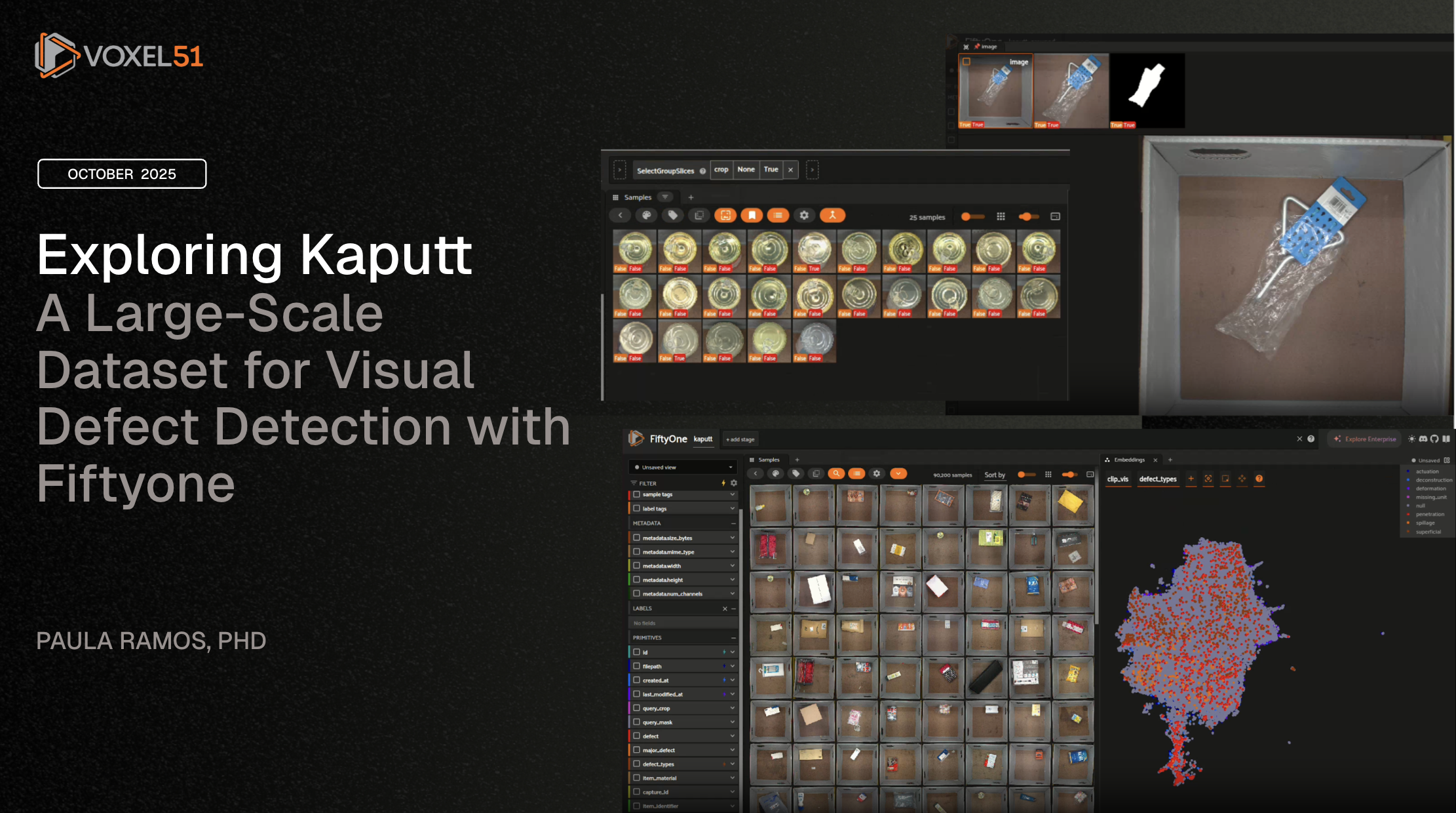
Dataset: [kaputt-dataset.com](https://www.kaputt-dataset.com)
Reference: *Kaputt: A Large-Scale Benchmark for Visual Defect Detection in Retail Logistics* (ICCV 2025)
**So, what’s the takeaway?**
1. Load and explore the **Kaputt dataset** interactively using FiftyOne.
2. Visualize its structure and metadata fields.
3. Compute and analyze embeddings, find similar samples query and filter the dataset from different inputs.
4. Experiment with VLMs as **FastVLM** and other models from the FiftyOne Model Zoo.
5. Demonstrate how FiftyOne helps uncover valuable insights into data quality, bias, and model performance.
## Setup
If you haven’t already, install the required packages. These cells will only install packages if they’re missing. This notebook was tested in a Python Env (py 3.10)
### Request access and download the dataset locally and dataset structure
1. **Fill the Request** [Form](https://www.kaputt-dataset.com/)
- Locate the access form for the Kaputt dataset, available on the dataset’s official website or publication page.
- Complete all required fields with accurate information such as your **name**, **email**, and **affiliation**.
2. **Submit the Form**
- Double-check your details before submission.
- Click **Submit** to send your access request.
3. **Check Your Email**
- Open the inbox of the email address you provided.
- Look for a confirmation or dataset access message.
#### Dataset structure
In this notebook we will explore the complete query folder, for the other folders you can extend with the provided code.
```none
kaputt/
├── datasets/ # Parquet metadata (index tables)
│ ├── query-train.parquet
│ ├── query-validation.parquet
│ ├── query-test.parquet
│ ├── reference-train.parquet
│ ├── reference-validation.parquet
│ ├── reference-test.parquet
│ └── README.md
│
├── query-image/ # Full query images (main inputs)
│ └── data/
│ ├── train/
│ │ └── query-data/image/
│ │ ├── .jpg
│ │ ├── ...
│ ├── validation/
│ │ └── query-data/image/
│ │ ├── .jpg
│ │ ├── ...
│ └── test/
│ └── query-data/image/
│ ├── .jpg
│ ├── ...
│
├── query-crop/ # Cropped item regions
│ └── data/
│ ├── train/
│ │ └── query-data/crop/
│ │ ├── .jpg
│ │ ├── ...
│ ├── validation/
│ │ └── query-data/crop/
│ │ ├── .jpg
│ │ ├── ...
│ └── test/
│ └── query-data/crop/
│ ├── .jpg
│ ├── ...
│
├── query-mask/ # Binary/segmentation masks
│ └── data/
│ ├── train/
│ │ └── query-data/mask/
│ │ ├── .png
│ │ ├── ...
│ ├── validation/
│ │ └── query-data/mask/
│ │ ├── .png
│ │ ├── ...
│ └── test/
│ └── query-data/mask/
│ ├── .png
│ ├── ...
│
├── reference-image/ # Reference (non-defective) images
│ └── data/
│ ├── train/reference-data/image/
│ ├── validation/reference-data/image/
│ └── test/reference-data/image/
│
├── reference-crop/ # Crops for reference images
│ └── data/
│ ├── train/reference-data/crop/
│ ├── validation/reference-data/crop/
│ └── test/reference-data/crop/
│
├── reference-mask/ # Segmentation masks for reference images
│ └── data/
│ ├── train/reference-data/mask/
│ ├── validation/reference-data/mask/
│ └── test/reference-data/mask/
│
├── sample-data/ # Small subset for testing
│ ├── data/
│ │ └── train/
│ │ ├── query-data/
│ │ │ ├── image/
│ │ │ ├── crop/
│ │ │ └── mask/
│ │ └── reference-data/
│ │ ├── image/
│ │ ├── crop/
│ │ └── mask/
│ ├── query-sample.parquet
│ └── reference-sample.parquet
│
└── kaputt-release/ # Original release version (mirrors structure above)
├── train/
│ ├── query-data/
│ └── reference-data/
├── validation/
│ ├── query-data/
│ └── reference-data/
└── test/
├── query-data/
└── reference-data/
```
### Import Kaputt (Query Only)
This cell imports the query portion of the Kaputt dataset into FiftyOne. It reads the query Parquet files from `/datasets/`, builds absolute paths for images, crops, and masks, and creates a FiftyOne dataset with fields for defect attributes and item metadata. Only train and validation splits are loaded for faster testing.
## Create and Save FiftyOne Dataset
This cell creates a new FiftyOne dataset named after DATASET_NAME, adds samples for each available split (train and validation), and computes image metadata (dimensions, channels, etc.). If a dataset with the same name already exists, it is replaced to ensure a clean import.
**After adding all samples:**
- The dataset is saved and marked as persistent.
- Split counts are printed for verification.
- Metadata is computed in parallel using `NUM_WORKERS_METADATA`
### Compute CLIP Embeddings and Similarity Index
This cell uses the `CLIP ViT-B/32` model from the **FiftyOne Model Zoo** to generate visual embeddings for all samples in the dataset. The embeddings are stored in the field `clip_embeddings` and used to build a similarity index (`clip_sim`) via the **FiftyOne Brain** module.
This enables efficient image similarity search, semantic clustering, and content-based exploration directly within FiftyOne.
### Dimensionality Reduction with UMAP
This cell applies **UMAP** `(Uniform Manifold Approximation and Projection)` to the CLIP embeddings stored in `clip_embeddings`. It computes a 2D visualization of the dataset’s feature space using the FiftyOne Brain module and saves it under the key `clip_vis`.
This allows interactive exploration of the dataset in embedding space, revealing visual clusters and relationships between samples.
### Create Index for Faster Filtering
This cell creates a compound index on the fields `defect_types`, `item_material`, and `split` to optimize query performance in FiftyOne. By indexing these commonly filtered fields, dataset operations such as searching, filtering, and aggregating by defect category or material type become significantly faster, especially when working with **large datasets**.
Open a web browser session to play interactively with your dataset, metadata and embeddings.
### Explore visually in the FiftyOne App
## Apply FastVLM to Evaluate Defect Severity
This cells integrate the `FastVLM` model from the **open-source community** into FiftyOne to analyze the Kaputt dataset. It registers the model source from GitHub, downloads the desired FastVLM variant (`0.5B`, `1.5B`, or `7B`), and loads it into the environment.
Using a detailed prompt adapted from the model authors, the system asks the model to reason about item condition and defect severity. The model’s output is stored in a new field called result, containing structured JSON with:
`"condition"` → `"DAMAGED"` or `"UNDAMAGED"`
`"severity"` → Numeric score from 0 (`pristine`) to 10 (`completely destroyed`)
This enables analysis of how a large vision-language model interprets real-world packaging damage across the **Kaputt dataset**.
### Add predictions to your dataset
### Creating a Grouped Dataset with Images, Crops, and Masks in FiftyOne
This code demonstrates how to create a **grouped dataset** in FiftyOne, where each group can contain up to three related slices: the original image, a crop, and a mask. This structure is useful for organizing and visualizing multimodal or multiview data, such as associating each image with its corresponding crop and segmentation mask.
**Key steps:**
1. **Dataset Setup**:
- Checks if a grouped dataset with the specified name exists and deletes it if so.
- Creates a new grouped dataset and adds a group field (with `"image"` as the default slice).
2. **Sample Processing**:
- Iterates through each sample in the original dataset.
- Copies relevant fields (excluding system fields) to new grouped samples.
3. **Image Slice**:
- Always adds the original image as a slice in the group.
4. **Crop Slice**:
- If a crop is available (`sample.query_crop`), adds it as a separate slice.
5. **Mask Slice**:
- If a mask is available (`sample.query_mask`), reads and normalizes it to the 0-255 range.
- Applies a binary threshold to create a binarized mask.
- Only adds the mask slice if it contains meaningful (non-black) data.
6. **Debugging and Statistics**:
- Tracks and prints the number of total samples processed, masks added, and masks skipped.
- Prints a summary of the grouped dataset, including the number of mask samples.
This approach leverages FiftyOne’s native grouping feature, which is ideal for paired or multimodal data exploration and visualization. For more details on grouped datasets and their use cases, see the [FiftyOne grouped datasets documentation](https://docs.voxel51.com/user_guide/groups.html) and related [example notebooks](https://github.com/voxel51/fiftyone-examples/blob/master/examples/Grouped%20Datasets.ipynb).
> *Grouped datasets in FiftyOne allow you to organize related samples (such as images, masks, and crops) under a common group, enabling synchronized visualization and analysis across different data modalities or views.*
>
> [FiftyOne User Guide: Grouped Datasets](https://docs.voxel51.com/user_guide/groups.html)
>
### Computing Embeddings and Similarity Index for Crop Slices in FiftyOne
This code demonstrates how to compute embeddings for the “crop” slices in a grouped dataset and then create a similarity index for these crops using the CLIP model from the FiftyOne Model Zoo.
**Workflow:**
1. **Select Crop Slices:**
Use `select_group_slices("crop")` to create a flattened view containing only the crop samples from your grouped dataset.
2. **Load CLIP Model:**
Load the `"clip-vit-base32-torch"` model from the FiftyOne Model Zoo, which supports generating embeddings for images and patches [see: Model Zoo API Reference](https://docs.voxel51.com/model_zoo/api.html#generating-embeddings-with-zoo-models).
3. **Compute Embeddings:**
Compute embeddings for all crop samples and store them in the `"crop_embeddings"` field. This can be done using the `compute_embeddings()` method, which works with any model that exposes embeddings [see: Model Zoo API Reference](https://docs.voxel51.com/model_zoo/api.html#generating-embeddings-with-zoo-models).
4. **Create Similarity Index:**
Use `compute_similarity()` to create a similarity index over the crop samples, specifying the model and the field containing the precomputed embeddings. This enables similarity search and sorting by similarity for the crop slices [see: Creating an index](https://docs.voxel51.com/brain.html#creating-an-index).
### Visualizing Embeddings for Crop Slices in FiftyOne
This code demonstrates how to compute and visualize embeddings for the “crop” slices of a grouped dataset using FiftyOne Brain and the CLIP model.
**Steps:**
1. **Select Crop Slices:**
Use `select_group_slices("crop")` to obtain a flattened view containing only the crop samples from your grouped dataset.
2. **Compute Embeddings and Visualization:**
Call `fob.compute_visualization()` on the crop samples, specifying the CLIP model (`"clip-vit-base32-torch"`) and a `brain_key` to store the results. This function computes embeddings for each crop and projects them into a low-dimensional space (e.g., 2D) for visualization and interactive exploration in the FiftyOne App.
## Summary
- You explored your data and model predictions in FiftyOne
- You evaluated performance and inspected edge cases
- You identified concrete next steps to improve data/model quality
 Run in Google Colab
 View source on GitHub
 Download notebook